Binary Protected Attributes
TwoGroup.Rmd
library(FairnessTutorial)
library(dplyr)
library(corrplot)
library(randomForest)
library(pROC)
library(SpecsVerification)

data("mimic")
Data Preprocessing
Missing Data
# Calculate the number of missing values per column
missing_values <- sapply(mimic, function(x) sum(is.na(x)))

# Calculate the percentage of missing values per column
missing_values_percentage <- sapply(mimic, function(x) sum(is.na(x)) / length(x) * 100)

# Combine the results into a data frame for easy viewing
missing_data_summary <- data.frame(Number_of_Missing_Values = missing_values,
                                   Percentage = missing_values_percentage)

# Print the summary
print(missing_data_summary)
#>                    Number_of_Missing_Values  Percentage
#> aline_flg                                 0  0.00000000
#> icu_los_day                               0  0.00000000
#> hospital_los_day                          0  0.00000000
#> age                                       0  0.00000000
#> gender_num                                1  0.05630631
#> weight_first                            110  6.19369369
#> bmi                                     466 26.23873874
#> sapsi_first                              85  4.78603604
#> sofa_first                                6  0.33783784
#> service_unit                              0  0.00000000
#> service_num                               0  0.00000000
#> day_icu_intime                            0  0.00000000
#> day_icu_intime_num                        0  0.00000000
#> hour_icu_intime                           0  0.00000000
#> hosp_exp_flg                              0  0.00000000
#> icu_exp_flg                               0  0.00000000
#> day_28_flg                                0  0.00000000
#> mort_day_censored                         0  0.00000000
#> censor_flg                                0  0.00000000
#> sepsis_flg                                0  0.00000000
#> chf_flg                                   0  0.00000000
#> afib_flg                                  0  0.00000000
#> renal_flg                                 0  0.00000000
#> liver_flg                                 0  0.00000000
#> copd_flg                                  0  0.00000000
#> cad_flg                                   0  0.00000000
#> stroke_flg                                0  0.00000000
#> mal_flg                                   0  0.00000000
#> resp_flg                                  0  0.00000000
#> map_1st                                   0  0.00000000
#> hr_1st                                    0  0.00000000
#> temp_1st                                  3  0.16891892
#> spo2_1st                                  0  0.00000000
#> abg_count                                 0  0.00000000
#> wbc_first                                 8  0.45045045
#> hgb_first                                 8  0.45045045
#> platelet_first                            8  0.45045045
#> sodium_first                              5  0.28153153
#> potassium_first                           5  0.28153153
#> tco2_first                                5  0.28153153
#> chloride_first                            5  0.28153153
#> bun_first                                 5  0.28153153
#> creatinine_first                          6  0.33783784
#> po2_first                               186 10.47297297
#> pco2_first                              186 10.47297297
#> iv_day_1                                143  8.05180180
# remove columns with more than 10% missing data and impute the rest with median
# Identify columns with more than 10% missing values
columns_to_remove <- names(missing_values_percentage[missing_values_percentage > 10])

# Remove these columns
mimic <- select(mimic, -one_of(columns_to_remove))

# Impute remaining missing values with median
mimic<- mimic %>% mutate(across(where(~any(is.na(.))), ~ifelse(is.na(.), median(., na.rm = TRUE), .)))

# Check if there are any missing values left
remaining_missing_values <- sum(sapply(mimic, function(x) sum(is.na(x))))
remaining_missing_values
#> [1] 0Model Building
# Remove columns that are highly correlated with the outcome variable
corrplot(cor(select_if(mimic, is.numeric)), method = "color", tl.cex = 0.5)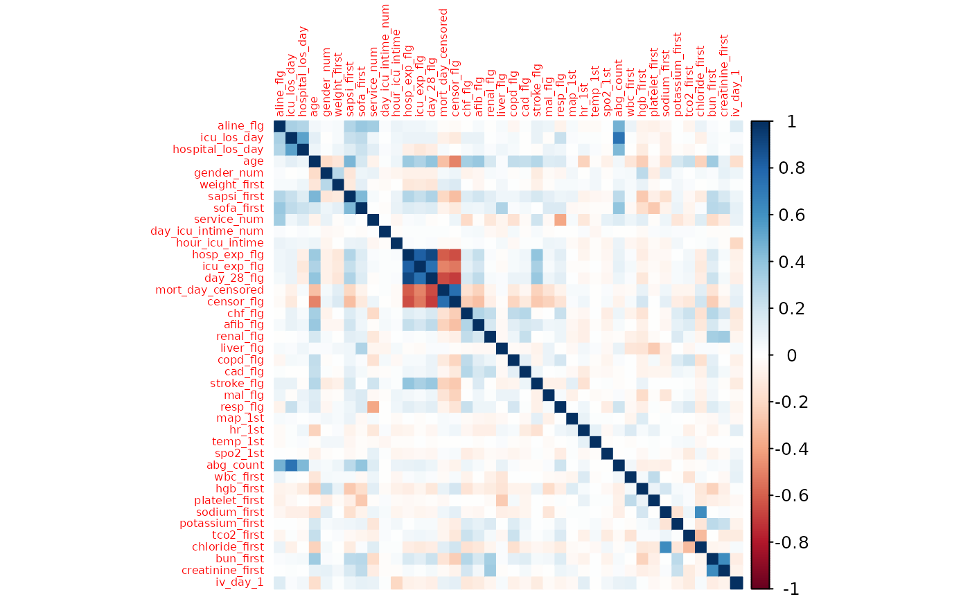
mimic <- mimic %>%
  select(-c("hosp_exp_flg", "icu_exp_flg", "mort_day_censored", "censor_flg"))

# Use 700 labels to train the mimic
train_data <- mimic %>% filter(row_number() <= 700)
# Fit a random forest model
set.seed(123)
rf_model <- randomForest(factor(day_28_flg) ~ ., data = train_data, ntree = 1000)

# Test the model on the remaining data
test_data <- mimic %>% filter(row_number() > 700)
test_data$pred <- predict(rf_model, newdata = test_data, type = "prob")[,2]
Fairness Evaluation
We will use sex as the sensitive attribute and day_28_flg as the outcome.
We choose threshold = 0.41 so that the overall FPR is around 5%.
cut_off <- 0.41

test_data %>%
  mutate(pred = ifelse(pred > cut_off, 1, 0)) %>%
  filter(day_28_flg == 0) %>%
  summarise(fpr = mean(pred))
#>          fpr
#> 1 0.05054945
Independence
Statistical Parity
eval_stats_parity(
  dat = test_data,
  outcome = "day_28_flg",
  group = "gender",
  probs = "pred",
  cutoff = cut_off
)
#> There is evidence that model does not satisfy statistical parity.
#>   Metric Group Female Group Male Difference  95% Diff CI Ratio 95% Ratio CI
#> 1    PPR         0.17       0.08       0.09 [0.05, 0.13]  2.12 [1.48, 3.05]
Conditional Statistical Parity
We conditional on age >= 60.
eval_cond_stats_parity(dat = test_data,
  outcome = "day_28_flg",
  group = "gender",
  probs = "pred",
  cutoff = cut_off,
  group2 = "age",
  condition = ">= 60")
#> There is evidence that model does not satisfy statistical parity.
#>   Metric Group Female Group Male Difference  95% Diff CI Ratio 95% Ratio CI
#> 1    PPR         0.34       0.21       0.13 [0.05, 0.21]  1.62 [1.18, 2.22]
We can also condition on a categorical variable. For example, we can condition on the service unit = MICU.
eval_cond_stats_parity(dat = test_data,
  outcome = "day_28_flg",
  group = "gender",
  probs = "pred",
  cutoff = cut_off,
  group2 = "service_unit",
  condition = "MICU")
#> There is not enough evidence that the model does not satisfy
#>             statistical parity.
#>   Metric Group Female Group Male Difference   95% Diff CI Ratio 95% Ratio CI
#> 1    PPR         0.15        0.1       0.05 [-0.01, 0.11]   1.5 [0.86, 2.61]
Separation
Equal Opportunity
eval_eq_opp(
  dat = test_data,
  outcome = "day_28_flg",
  group = "gender",
  probs = "pred",
  cutoff = cut_off
)
#> There is evidence that model does not satisfy equal opportunity.
#>   Metric GroupFemale GroupMale Difference    95% Diff CI Ratio 95% Ratio CI
#> 1    FNR        0.38      0.62      -0.24 [-0.39, -0.09]  0.61 [0.44, 0.85]
Predictive Equality
eval_pred_equality(
  dat = test_data,
  outcome = "day_28_flg",
  group = "gender",
  probs = "pred",
  cutoff = cut_off
)
#> There is evidence that model does not satisfy predictive
#>             equality.
#>   Metric GroupFemale GroupMale Difference  95% Diff CI Ratio 95% Ratio CI
#> 1    FPR        0.08      0.03       0.05 [0.02, 0.08]  2.67 [1.38, 5.14]
Balance for Positive Class
eval_pos_class_bal(
  dat = test_data,
  outcome = "day_28_flg",
  group = "gender",
  probs = "pred"
)
#> There is evidence that the model does not satisfy
#>             balance for positive class.
#>                 Metric GroupFemale GroupMale Difference  95% Diff CI Ratio
#> 1 Avg. Predicted Prob.        0.46      0.37       0.09 [0.04, 0.14]  1.24
#>   95% Ratio CI
#> 1 [1.09, 1.41]
Balance for Negative Class
eval_neg_class_bal(
  dat = test_data,
  outcome = "day_28_flg",
  group = "gender",
  probs = "pred"
)
#> There is enough evidence that the model does not satisfy
#>             balance for negative class.
#>                 Metric GroupFemale GroupMale Difference  95% Diff CI Ratio
#> 1 Avg. Predicted Prob.        0.15       0.1       0.05 [0.03, 0.07]   1.5
#>   95% Ratio CI
#> 1 [1.29, 1.74]
Sufficiency
Predictive Parity
eval_pred_parity(
  dat = test_data,
  outcome = "day_28_flg",
  group = "gender",
  probs = "pred",
  cutoff = cut_off
)
#> There is not enough evidence that the model does not satisfy
#>             predictive parity.
#>   Metric GroupFemale GroupMale Difference   95% Diff CI Ratio 95% Ratio CI
#> 1    PPV        0.62      0.66      -0.04 [-0.21, 0.13]  0.94 [0.72, 1.23]
Other Fairness Metrics
Brier Score Parity
eval_bs_parity(
  dat = test_data,
  outcome = "day_28_flg",
  group = "gender",
  probs = "pred"
)
#> There is not enough evidence that the model does not satisfy
#>             Brier Score parity.
#>        Metric GroupFemale GroupMale Difference   95% Diff CI Ratio 95% Ratio CI
#> 1 Brier Score        0.09      0.08       0.01 [-0.01, 0.03]  1.12 [0.89, 1.43]
Accuracy Parity
eval_acc_parity(
  dat = test_data,
  outcome = "day_28_flg",
  group = "gender",
  probs = "pred",
  cutoff = cut_off
)
#> There is not enough evidence that the model does not satisfy
#>             accuracy parity.
#>     Metric GroupFemale GroupMale Difference   95% Diff CI Ratio 95% Ratio CI
#> 1 Accuracy        0.87      0.88      -0.01 [-0.05, 0.03]  0.99 [0.94, 1.04]
Treatment Equality
eval_treatment_equality(
  dat = test_data,
  outcome = "day_28_flg",
  group = "gender",
  probs = "pred"
)
#> There is not enough evidence that the model does not satisfy
#>             treatment equality.
#>        Metric GroupFemale GroupMale Difference     95% Diff CI Ratio
#> 1 FN/FP Ratio        5.11      13.6      -8.49 [-33.33, 16.35]  0.38
#>   95% Ratio CI
#> 1  [0.1, 1.36]